MagicAdjuster Tutorial

This notebook demonstrates how to use the MagicAdjuster class for statistical distribution fitting and analysis.

Overview

MagicAdjuster is designed to:

• Fit statistical distributions to your data

• Perform goodness-of-fit tests (KS, Chi-square, RMSE)

• Provide seamless access to all SciPy distribution methods

• Run Monte Carlo stability analysis

Setup and Data Generation

Let’s start by importing the necessary libraries and generating some sample wind speed data.

import numpy as np
import matplotlib.pyplot as plt
import magica as ma
from magica.core import DataProcessor, MagicAdjuster

# Set random seed for reproducibility
np.random.seed(42)

# Generate sample wind speed data (Weibull-like distribution)
n_samples = 10000
wind_speeds = np.random.weibull(2, n_samples) * 8 + 2  # Scale and shift

# Plot histogram of wind speeds
plt.hist(wind_speeds, bins=30, color='skyblue', edgecolor='black')
plt.title('Histogram of Simulated Wind Speeds')
plt.xlabel('Wind Speed (m/s)')
plt.ylabel('Frequency')
plt.grid(True, alpha=0.3)
plt.show()

print(f"Generated {n_samples} wind speed measurements")
print(f"Min: {wind_speeds.min():.2f} m/s")
print(f"Max: {wind_speeds.max():.2f} m/s")
print(f"Mean: {wind_speeds.mean():.2f} m/s")
print(f"Std: {wind_speeds.std():.2f} m/s")

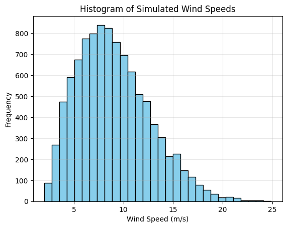
Generated 10000 wind speed measurements
Min: 2.03 m/s
Max: 24.87 m/s
Mean: 9.01 m/s
Std: 3.66 m/s

Basic Usage: Loading Data and Fitting a Distribution

# Load data using MagicA's DataProcessor
processor = ma.read_data(wind_speeds)
print(f"Loaded data: {processor}")

# Get basic statistics
stats = processor.get_basic_stats()
for key, value in stats.items():
    print(f"{key}: {value:.4f}")

Loaded data: DataProcessor(length=10000, dtype=float64)
count: 10000.0000
mean: 9.0101
std: 3.6634
var: 13.4203
min: 2.0273
max: 24.8700
median: 8.5888
q25: 6.2543
q75: 11.2852

# Fit a Weibull distribution (common for wind data)
processor.fit_distribution('weibull_min')
print(f"Updated processor: {processor}")

# Get fitted parameters
params = processor.get_fitted_params()
print(f"\nFitted Weibull parameters:")
print(f"Shape (c): {params[0]:.4f}")
print(f"Location (loc): {params[1]:.4f}")
print(f"Scale: {params[2]:.4f}")

# Get distribution info
info = processor.get_distribution_info()
print(f"\nDistribution info:")
for key, value in info.items():
    print(f"{key}: {value}")

Updated processor: DataProcessor(length=10000, dtype=float64, distribution='weibull_min')

Fitted Weibull parameters:
Shape (c): 2.0109
Location (loc): 1.9748
Scale: 7.9409

Distribution info:
name: weibull_min
parameters: (np.float64(2.0108828522203734), np.float64(1.9747913720744723), np.float64(7.940931128156864))
num_params: 3
data_size: 10000

Accessing SciPy Methods Directly

Once a distribution is fitted, you can access all SciPy distribution methods directly through the processor.

# Smart defaults: evaluate at original data points
pdf_values = processor.pdf()  # PDF at all original data points
cdf_values = processor.cdf()  # CDF at all original data points

print(f"PDF values (first 10): {pdf_values[:10]}")
print(f"CDF values (first 10): {cdf_values[:10]}")

# Custom inputs also work
prob_10ms = processor.cdf(10.0)  # P(wind speed ≤ 10 m/s)
percentile_95 = processor.ppf(0.95)  # 95th percentile wind speed

print(f"\nP(wind speed ≤ 10 m/s): {prob_10ms:.4f}")
print(f"95th percentile wind speed: {percentile_95:.2f} m/s")

# Generate random samples from fitted distribution
random_samples = processor.rvs(size=5)
print(f"5 random wind speed samples: {random_samples}")

PDF values (first 10): [0.10833923 0.02040302 0.07653296 0.09622977 0.0882     0.08819511
 0.05855587 0.04647147 0.09595044 0.08076123]
CDF values (first 10): [0.38044565 0.95426667 0.73969983 0.60636965 0.15898947 0.15896499
 0.05952766 0.87233822 0.60883529 0.71586528]

P(wind speed ≤ 10 m/s): 0.6399
95th percentile wind speed: 15.68 m/s
5 random wind speed samples: [7.41742125 7.03970835 5.48590614 9.65316876 8.37195175]

Goodness-of-Fit Testing

Evaluate how well the distribution fits your data using various statistical tests.

# Kolmogorov-Smirnov test
ks_result = processor.goodness_of_fit('ks')
print("Kolmogorov-Smirnov Test:")
print(f"  Statistic: {ks_result['ks_statistic']:.6f}")
print(f"  P-value: {ks_result['p_value']:.6f}")
print(f"  Result: {'Good fit' if ks_result['p_value'] > 0.05 else 'Poor fit'} (α = 0.05)")

# Chi-square test
chi2_result = processor.goodness_of_fit('chi2')
print("\nChi-square Test:")
print(f"  Statistic: {chi2_result['chi2_statistic']:.6f}")
print(f"  P-value: {chi2_result['p_value']:.6f}")
print(f"  Bins used: {chi2_result['n_bins']}")
print(f"  Result: {'Good fit' if chi2_result['p_value'] > 0.05 else 'Poor fit'} (α = 0.05)")

# RMSE
rmse = processor.goodness_of_fit('rmse')
print(f"\nRoot Mean Square Error: {rmse:.6f}")

Kolmogorov-Smirnov Test:
  Statistic: 0.005025
  P-value: 0.961225
  Result: Good fit (α = 0.05)

Chi-square Test:
  Statistic: 13.724140
  P-value: 0.746889
  Bins used: 19
  Result: Good fit (α = 0.05)

Root Mean Square Error: 0.001775

/Users/danilocoutodesouza/Documents/Programs_and_scripts/MagicA/magica/core/magic_adjuster.py:467: UserWarning: Normalizing expected frequencies. Original sum: 9997.357954, Target sum: 10000
  warnings.warn(f"Normalizing expected frequencies. Original sum: {expected_freq.sum():.6f}, "

Understanding Chi-square Test and Number of Bins

The chi-square goodness-of-fit test compares observed frequencies in histogram bins with expected frequencies from the fitted distribution. The number of bins significantly affects the test results.

# Demonstrate different binning methods for chi-square test
binning_methods = ['doane', 'sturges', 'freedman-diaconis', 'rice', 'scott', 30]

print("Chi-square Test Results with Different Binning Methods:")
print("-" * 70)
print(f"{'Method':<20} {'Bins':<6} {'Chi2 Stat':<12} {'P-value':<12} {'Result'}")
print("-" * 70)

for method in binning_methods:
    chi2_result = processor.goodness_of_fit('chi2', bins=method)
    result_text = 'Good fit' if chi2_result['p_value'] > 0.05 else 'Poor fit'
    method_name = str(method) if isinstance(method, int) else method

    print(f"{method_name:<20} {chi2_result['n_bins']:<6} {chi2_result['chi2_statistic']:<12.4f} "
          f"{chi2_result['p_value']:<12.6f} {result_text}")

print("\nBinning Method Guidelines:")
print("- Doane: Best for skewed distributions (default)")
print("- Sturges: Good for normal distributions, conservative")
print("- Freedman-Diaconis: Robust for various distributions")
print("- Rice: Simple rule, scales with cube root of sample size")
print("- Scott: Minimizes integrated mean square error")
print("- Fixed number: Use when you need specific bin count")

Chi-square Test Results with Different Binning Methods:
----------------------------------------------------------------------
Method               Bins   Chi2 Stat    P-value      Result
----------------------------------------------------------------------
doane                19     13.7241      0.746889     Good fit
sturges              14     9.7122       0.717285     Good fit
freedman-diaconis    48     39.3616      0.777948     Good fit
rice                 43     40.2136      0.549608     Good fit
scott                38     31.4205      0.727675     Good fit
30                   30     29.8675      0.420640     Good fit

Binning Method Guidelines:
- Doane: Best for skewed distributions (default)
- Sturges: Good for normal distributions, conservative
- Freedman-Diaconis: Robust for various distributions
- Rice: Simple rule, scales with cube root of sample size
- Scott: Minimizes integrated mean square error
- Fixed number: Use when you need specific bin count

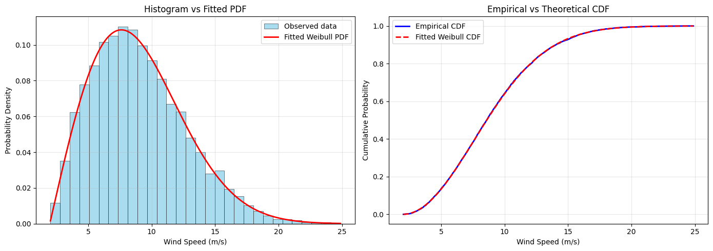
Visualization: Comparing Data and Fitted Distribution

# Create comparison plots
fig, (ax1, ax2) = plt.subplots(1, 2, figsize=(14, 5))

# Plot 1: Histogram with fitted PDF
ax1.hist(wind_speeds, bins=30, density=True, alpha=0.7, color='skyblue',
         label='Observed data', edgecolor='black', linewidth=0.5)

# Generate smooth curve for fitted distribution
x_smooth = np.linspace(wind_speeds.min(), wind_speeds.max(), 1000)
pdf_smooth = processor.pdf(x_smooth)
ax1.plot(x_smooth, pdf_smooth, 'r-', linewidth=2, label='Fitted Weibull PDF')

ax1.set_xlabel('Wind Speed (m/s)')
ax1.set_ylabel('Probability Density')
ax1.set_title('Histogram vs Fitted PDF')
ax1.legend()
ax1.grid(True, alpha=0.3)

# Plot 2: Empirical vs Theoretical CDF
sorted_data = np.sort(wind_speeds)
empirical_cdf = np.arange(1, len(sorted_data) + 1) / len(sorted_data)
theoretical_cdf = processor.cdf(sorted_data)

ax2.plot(sorted_data, empirical_cdf, 'b-', linewidth=2, label='Empirical CDF')
ax2.plot(sorted_data, theoretical_cdf, 'r--', linewidth=2, label='Fitted Weibull CDF')

ax2.set_xlabel('Wind Speed (m/s)')
ax2.set_ylabel('Cumulative Probability')
ax2.set_title('Empirical vs Theoretical CDF')
ax2.legend()
ax2.grid(True, alpha=0.3)

plt.tight_layout()
plt.show()

Using Different Distributions

Let’s try fitting other distributions to see which one works best.

# Test different distributions
distributions_to_test = ['weibull_min', 'lognorm', 'gamma', 'norm', 'expon']
results = []

for dist_name in distributions_to_test:
    # Create a fresh processor for each distribution
    temp_processor = ma.read_data(wind_speeds)
    temp_processor.fit_distribution(dist_name)

    # Calculate goodness-of-fit metrics
    ks_test = temp_processor.goodness_of_fit('ks')
    rmse = temp_processor.goodness_of_fit('rmse')

    results.append({
        'distribution': dist_name,
        'ks_pvalue': ks_test['p_value'],
        'rmse': rmse,
        'parameters': temp_processor.get_fitted_params()
    })

# Display results
print("Distribution Comparison:")
print("-"  60)
print(f"{'Distribution':<15} {'KS p-value':<12} {'RMSE':<10} {'Fit Quality'}")
print("-"  60)

for result in results:
    quality = "Good" if result['ks_pvalue'] > 0.05 else "Poor"
    print(f"{result['distribution']:<15} {result['ks_pvalue']:<12.6f} {result['rmse']:<10.6f} {quality}")

# Find best distribution (highest KS p-value)
best_result = max(results, key=lambda x: x['ks_pvalue'])
print(f"\nBest distribution: {best_result['distribution']} (KS p-value: {best_result['ks_pvalue']:.6f})")

Distribution Comparison:
------------------------------------------------------------
Distribution    KS p-value   RMSE       Fit Quality
------------------------------------------------------------
weibull_min     0.961225     0.001775   Good
lognorm         0.007746     0.010314   Poor
gamma           0.020087     0.009206   Poor
norm            0.000000     0.029975   Poor
expon           0.000000     0.134458   Poor

Best distribution: weibull_min (KS p-value: 0.961225)

Advanced Usage: Distribution Parameters with Constraints

You can constrain distribution parameters during fitting (e.g., fix location parameter).

# Fit Weibull with fixed location parameter (floc=0)
processor_constrained = ma.read_data(wind_speeds)
processor_constrained.fit_distribution('weibull_min', floc=0)  # Fix location to 0

params_constrained = processor_constrained.get_fitted_params()
print("Weibull with floc=0:")
print(f"Shape (c): {params_constrained[0]:.4f}")
print(f"Location (fixed): {params_constrained[1]:.4f}")
print(f"Scale: {params_constrained[2]:.4f}")

# Compare with unconstrained fit
params_unconstrained = processor.get_fitted_params()
print("\nUnconstrained Weibull:")
print(f"Shape (c): {params_unconstrained[0]:.4f}")
print(f"Location: {params_unconstrained[1]:.4f}")
print(f"Scale: {params_unconstrained[2]:.4f}")

# Compare goodness of fit
ks_constrained = processor_constrained.goodness_of_fit('ks')
ks_unconstrained = processor.goodness_of_fit('ks')

print(f"\nGoodness of fit comparison:")
print(f"Constrained KS p-value: {ks_constrained['p_value']:.6f}")
print(f"Unconstrained KS p-value: {ks_unconstrained['p_value']:.6f}")

Weibull with floc=0:
Shape (c): 2.6326
Location (fixed): 0.0000
Scale: 10.1575

Unconstrained Weibull:
Shape (c): 2.0109
Location: 1.9748
Scale: 7.9409

Goodness of fit comparison:
Constrained KS p-value: 0.000000
Unconstrained KS p-value: 0.961225

Monte Carlo Stability Analysis

Determine the minimum sample size needed for stable parameter estimation using standard Monte Carlo analysis.

Large Sample Size Effect and Monte Carlo CPS Method

The Problem with Large Datasets

When working with very large datasets (>10,000 samples), statistical tests become extremely powerful, making p-values very small even for practically negligible effects. This phenomenon is known as the “large sample size effect.”

Let’s demonstrate this problem and show how the Monte Carlo CPS (Coefficient/P-value/Sample size) method can help.

# Generate large synthetic dataset for demonstrating large sample size effect
print("Generating large synthetic dataset for demonstration...")
print("(This simulates the 'large sample size effect' with synthetic data)\n")

# Generate 10 years of hourly data (87,600 samples)
from magica.utils import generate_wind_data

wind_speeds_large = generate_wind_data(
    n_years=10,
    freq='H',  # Hourly data
    mean_wind=8.0,
    weibull_shape=2.0,
    seasonal_amplitude=0.3,
    n_storms_per_year=5,
    storm_duration_range=(12, 48),  # 12-48 hour storms
    storm_intensity_range=(15, 25),
    random_seed=42
)

# Convert Series to array
wind_speeds_real = wind_speeds_large.values
large_sample_size = len(wind_speeds_real)

print(f"Generated synthetic dataset: {large_sample_size:,} samples")
print(f"Mean: {wind_speeds_real.mean():.2f} m/s")
print(f"Std: {wind_speeds_real.std():.2f} m/s")

# Fit Weibull distribution to large dataset
large_processor = ma.read_data(wind_speeds_real)
large_processor.fit_distribution('weibull_min')

# Compare goodness-of-fit tests between small and large datasets
print("\n" + "="*60)
print("COMPARISON: Small vs Large Dataset")
print("="*60)

Generating large synthetic dataset for demonstration...
(This simulates the 'large sample size effect' with synthetic data)

Generated synthetic dataset: 87,625 samples
Mean: 7.62 m/s
Std: 3.52 m/s

/Users/danilocoutodesouza/Documents/Programs_and_scripts/MagicA/magica/utils/synthetic_data.py:117: FutureWarning: 'H' is deprecated and will be removed in a future version, please use 'h' instead.
  dates = pd.date_range(start=start_date, end=dates[-1], freq=freq)

============================================================
COMPARISON: Small vs Large Dataset
============================================================

The Monte Carlo CPS Solution

The Monte Carlo CPS method addresses this by:

1. Testing multiple subsample sizes to understand how fit quality evolves

2. Using RMSE as the primary stability indicator - it shows clear, smooth convergence

3. Finding the optimal sample size where RMSE stabilizes (point of diminishing returns)

4. Providing interpretable quality metrics at the recommended sample size

Why RMSE is the best indicator:

• Shows smooth, monotonic decrease as sample size increases

• Clear “elbow” point where improvements become negligible

• More reliable than p-values which can be erratic

• Directly measures fit quality improvement

Let’s run a comprehensive analysis focused on RMSE stability:

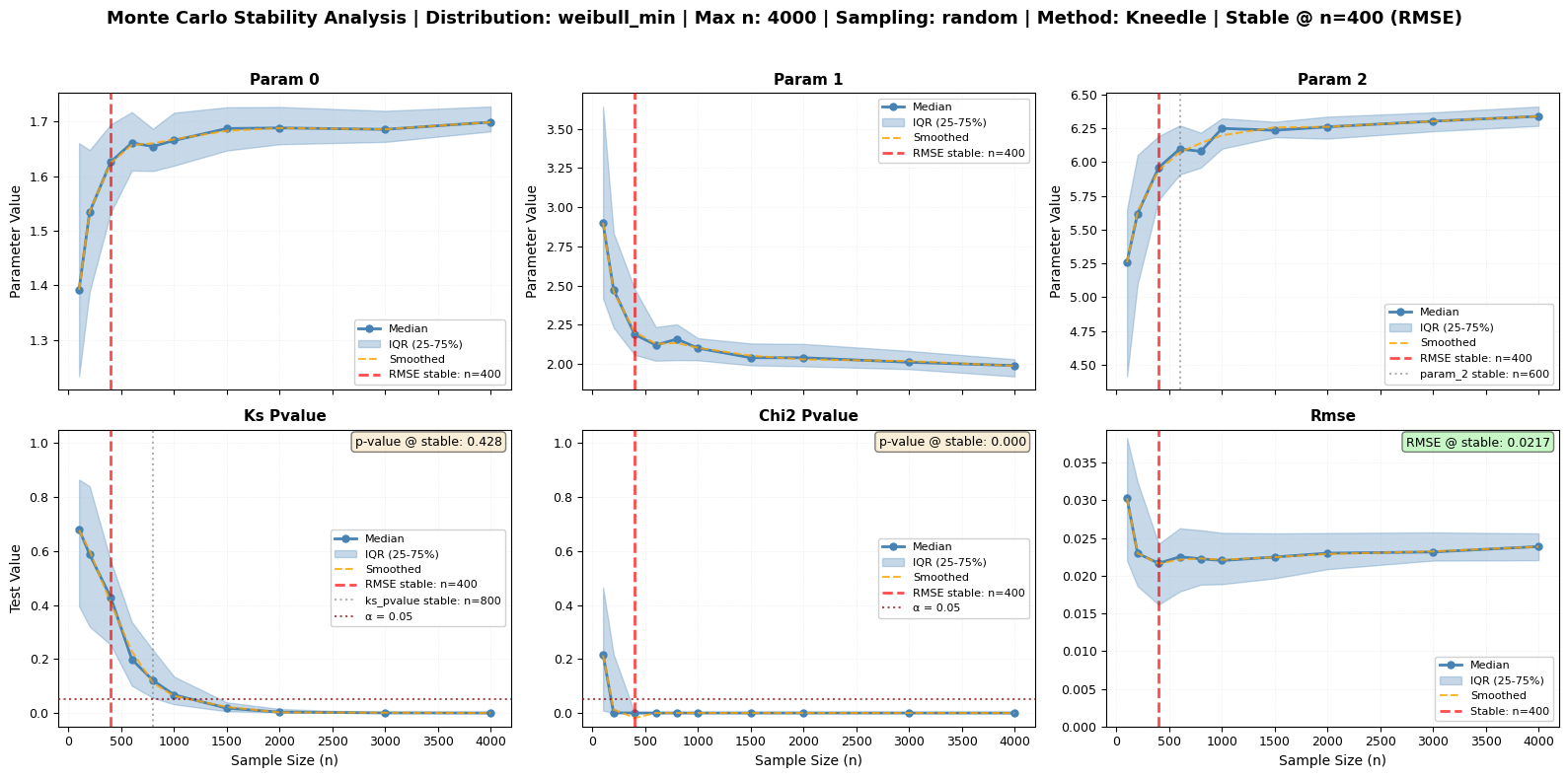
# Run comprehensive Monte Carlo CPS analysis with RMSE-focused stability detection
print("Running Monte Carlo CPS Analysis on Large Dataset...")
print("This will take a moment as we test multiple subsample sizes...\n")

# Define the sample sizes to test (from small to large)
test_sizes = [100, 200, 400, 600, 800, 1000, 1500, 2000, 3000, 4000]

# ⭐ KEY CONFIGURATION: Use Kneedle method for RMSE stability detection
# Kneedle excels at finding the "elbow" in decreasing RMSE curves
mc_results = large_processor.monte_carlo_fit(
    sizes=test_sizes,                    # Sample sizes to test
    n_repeats=50,                        # Number of subsamples per size
    tests=['ks', 'chi2', 'rmse'],        # Include all tests (RMSE is primary)
    stability_method='kneedle',          # ⭐ Best for RMSE stability detection
    smooth=True,                         # Smooth curves for clearer elbow detection
    sampling='random',                   # Sampling strategy
    seed=42,                             # For reproducibility
    fig_output_path='cps_analysis.png',  # Auto-generate figure with RMSE focus
    plot_type='series'                   # Series plot style
)

print("✓ Monte Carlo CPS analysis completed!")
print(f"Results dimensions: {dict(mc_results.dims)}")
print(f"Available variables: {list(mc_results.data_vars.keys())}")
print(f"Figure saved to: {mc_results.attrs['figure_path']}")

# Get the recommended size (based on RMSE with Kneedle method)
recommended_n = mc_results.attrs['recommended_size']
primary_metric = mc_results.attrs['primary_metric']

print(f"\n{'='*60}")
print("⭐ STABILITY ANALYSIS RESULTS (RMSE-Focused)")
print("="*60)

if recommended_n is not None:
    print(f"✓ {primary_metric.upper()} stabilizes at n = {recommended_n} (RECOMMENDED)")
    print(f"  Detection method: Kneedle algorithm (optimal for RMSE)")

    # Show quality metrics at the stable point
    if mc_results.attrs.get('stable_rmse') is not None:
        print(f"  RMSE at stable point: {mc_results.attrs['stable_rmse']:.6f}")
    if mc_results.attrs.get('stable_pvalue_ks') is not None:
        print(f"  KS p-value at stable point: {mc_results.attrs['stable_pvalue_ks']:.4f}")
else:
    print(f"○ {primary_metric.upper()}: no clear stability detected")

# Show other stability points as examples (not the focus)
print(f"\nOther metrics (for reference only):")
stability_info = mc_results.attrs['stability_points']
for param in ['param_0', 'param_2', 'ks_pvalue', 'chi2_pvalue']:
    if param in stability_info:
        info = stability_info[param]
        size = info.get('size', 'Not detected')
        print(f"  {param}: n = {size}")

print(f"\n{'='*60}")
print("💡 FOCUS ON RMSE:")
print("  • RMSE shows the clearest convergence pattern")
print("  • Kneedle algorithm finds the optimal 'elbow' point")
print("  • Other metrics shown for completeness but less reliable")
print(f"  • Use n = {recommended_n} for robust inference")

Running Monte Carlo CPS Analysis on Large Dataset...
This will take a moment as we test multiple subsample sizes...

Monte Carlo sizes:   0%|          | 0/10 [00:00<?, ?it/s]/Users/danilocoutodesouza/miniconda3/envs/magica/lib/python3.11/site-packages/scipy/stats/_stats_py.py:7400: RuntimeWarning: divide by zero encountered in divide
  terms = (f_obs - f_exp)**2 / f_exp
Monte Carlo sizes: 100%|██████████| 10/10 [00:12<00:00,  1.24s/it]

✓ Monte Carlo CPS analysis completed!
Results dimensions: {'sizes': 10, 'repeats': 50}
Available variables: ['param_0', 'param_1', 'param_2', 'ks_statistic', 'ks_pvalue', 'chi2_statistic', 'chi2_pvalue', 'rmse']
Figure saved to: cps_analysis.png

============================================================
⭐ STABILITY ANALYSIS RESULTS (RMSE-Focused)
============================================================
✓ RMSE stabilizes at n = 400 (RECOMMENDED)
  Detection method: Kneedle algorithm (optimal for RMSE)
  RMSE at stable point: 0.021654
  KS p-value at stable point: 0.4281

Other metrics (for reference only):
  param_0: n = 400
  param_2: n = 600
  ks_pvalue: n = 800
  chi2_pvalue: n = 400

============================================================
💡 FOCUS ON RMSE:
  • RMSE shows the clearest convergence pattern
  • Kneedle algorithm finds the optimal 'elbow' point
  • Other metrics shown for completeness but less reliable
  • Use n = 400 for robust inference

/var/folders/bh/y994_xnx7kg9z0q_bglc3sbm0000gn/T/ipykernel_9133/3474790011.py:23: FutureWarning: The return type of `Dataset.dims` will be changed to return a set of dimension names in future, in order to be more consistent with `DataArray.dims`. To access a mapping from dimension names to lengths, please use `Dataset.sizes`.
  print(f"Results dimensions: {dict(mc_results.dims)}")

# Display key results
recommended_n = mc_results.attrs['recommended_size']
primary_metric = mc_results.attrs['primary_metric']

print(f"\n{'='*60}")
print(f"Recommended sample size: n = {recommended_n}")
print(f"Based on: {primary_metric.upper()}")

if mc_results.attrs.get('stable_rmse') is not None:
    print(f"\nQuality at stable point:")
    print(f"  RMSE: {mc_results.attrs['stable_rmse']:.6f}")
if mc_results.attrs.get('stable_pvalue_ks') is not None:
    print(f"  KS p-value: {mc_results.attrs['stable_pvalue_ks']:.4f}")
print(f"{'='*60}")

============================================================
Recommended sample size: n = 400
Based on: RMSE

Quality at stable point:
  RMSE: 0.021654
  KS p-value: 0.4281
============================================================

📊 Interpreting the CPS Analysis Figure

⭐ Primary Focus: RMSE Panel (Bottom Right)

The RMSE panel is your main indicator for stability detection:

• Orange dashed line: Smoothed RMSE curve showing convergence pattern

• Red vertical line: Detected stability point (the optimal sample size)

• Pattern: Decreasing RMSE that flattens after the stability point

Other Panels (shown for completeness):

• Top row: Parameter convergence (shape, scale, location)

• Bottom left/center: Statistical test p-values (can be erratic)

Key Takeaway: Use the RMSE stability point as your recommended sample size for robust inference.

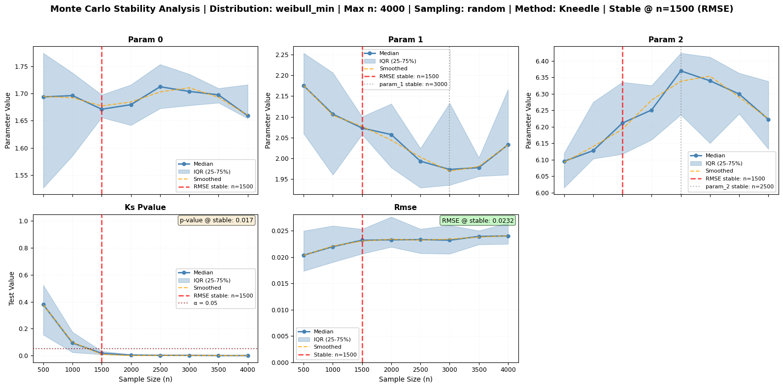
Monte Carlo Sampling Strategies

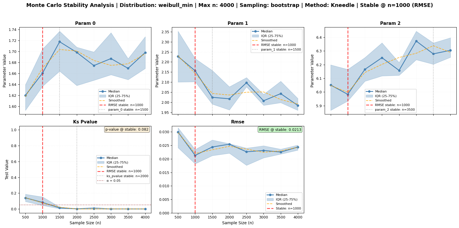
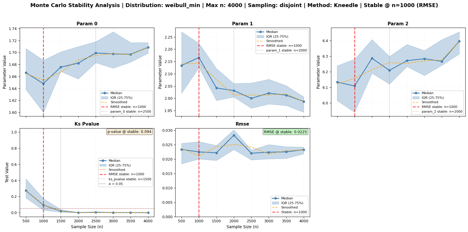
The monte_carlo_fit method offers different sampling strategies. Let’s compare them while maintaining our focus on RMSE stability detection as the primary indicator:

# Compare different sampling strategies with RMSE-focused stability detection
# Using smaller sizes and fewer repeats for demonstration purposes
sampling_strategies = ['random', 'bootstrap', 'disjoint']
strategy_results = {}

print("Comparing Monte Carlo Sampling Strategies (RMSE-Focused):")
print("=" * 60)
print("NOTE: Using reduced parameters for demonstration (faster execution)")
print("      Always focusing on RMSE as primary stability indicator")
print("")

for i, strategy in enumerate(sampling_strategies):
    print(f"\nTesting '{strategy}' sampling...")

    # Run analysis with Kneedle method for RMSE stability
    fig_path = f'mc_sampling_{strategy}.png'

    mc_strategy = large_processor.monte_carlo_fit(
        sizes=[500, 1000, 1500, 2000, 2500, 3000, 3500, 4000],
        n_repeats=10,  # Reduced for speed
        tests=['ks', 'rmse'],          # Focus on RMSE
        stability_method='kneedle',    # ⭐ Best for RMSE
        smooth=True,                   # Smooth for clear elbow
        sampling=strategy,
        seed=42,
        fig_output_path=fig_path,
        plot_type='series'
    )

    strategy_results[strategy] = mc_strategy

    # Get recommended size (based on RMSE)
    recommended_n = mc_strategy.attrs.get('recommended_size', 'Not detected')
    primary_metric = mc_strategy.attrs.get('primary_metric', 'rmse')

    print(f"  ⭐ {primary_metric.upper()} stability: n = {recommended_n} (PRIMARY)")

    # Show parameters as examples only
    stability = mc_strategy.attrs['stability_points']
    if 'param_0' in stability:
        param_0_size = stability['param_0'].get('size', 'Not detected')
        print(f"  • Shape parameter: n = {param_0_size} (example)")

    print(f"  Figure saved to: {mc_strategy.attrs['figure_path']}")
    print(f"  ✓ Completed")

print("\n" + "="*60)
print("SAMPLING STRATEGY GUIDE:")
print("="*60)
print("🎲 RANDOM sampling:")
print("   • Most common approach")
print("   • Each subsample is independently drawn without replacement")
print("   • Good for general stability analysis")
print("   • May have higher variance between subsamples")
print("")
print("🔄 BOOTSTRAP sampling:")
print("   • Samples with replacement")
print("   • Useful for uncertainty quantification")
print("   • Can help assess sampling distribution")
print("   • Good for confidence interval estimation")
print("   • Allows subsample size > original data size")
print("")
print("📐 DISJOINT sampling (use sampling='disjoint'):")
print("   • Creates non-overlapping partitions")
print("   • Each data point used exactly once per size")
print("   • More representative of data structure")
print("   • Lower variance, more reproducible")
print("   • Good when data has temporal/spatial order")
print("")
print("💡 RECOMMENDATION:")
print("   Start with 'random' for general use, try 'disjoint' for ordered data")
print("")
print("⭐ REMEMBER:")
print("   • All strategies use RMSE as primary stability indicator")
print("   • Look at the RMSE panel (rightmost) in the figures")
print("   • Parameter stability shown as examples, not the focus")
print("")
print("⚡ PERFORMANCE TIP:")
print("   For production analysis, use n_repeats=30-50 and more sample sizes.")
print("   This demo uses reduced parameters for faster execution.")

# Display comparison summary
print("\n" + "="*60)
print("Generated figures comparing sampling strategies:")
print("⭐ Focus on RMSE panel (bottom right) in each figure")
for strategy, results in strategy_results.items():
    recommended = results.attrs.get('recommended_size', 'N/A')
    print(f"  - {strategy}: n = {recommended} | {results.attrs['figure_path']}")

Comparing Monte Carlo Sampling Strategies (RMSE-Focused):
============================================================
NOTE: Using reduced parameters for demonstration (faster execution)
      Always focusing on RMSE as primary stability indicator


Testing 'random' sampling...

Monte Carlo sizes: 100%|██████████| 8/8 [00:02<00:00,  2.85it/s]

  ⭐ RMSE stability: n = 1500 (PRIMARY)
  • Shape parameter: n = 1500 (example)
  Figure saved to: mc_sampling_random.png
  ✓ Completed

Testing 'bootstrap' sampling...

Monte Carlo sizes: 100%|██████████| 8/8 [00:02<00:00,  2.97it/s]

  ⭐ RMSE stability: n = 1000 (PRIMARY)
  • Shape parameter: n = 1500 (example)
  Figure saved to: mc_sampling_bootstrap.png
  ✓ Completed

Testing 'disjoint' sampling...

Monte Carlo sizes: 100%|██████████| 8/8 [00:02<00:00,  2.97it/s]

  ⭐ RMSE stability: n = 1000 (PRIMARY)
  • Shape parameter: n = 2500 (example)
  Figure saved to: mc_sampling_disjoint.png
  ✓ Completed

============================================================
SAMPLING STRATEGY GUIDE:
============================================================
🎲 RANDOM sampling:
   • Most common approach
   • Each subsample is independently drawn without replacement
   • Good for general stability analysis
   • May have higher variance between subsamples

🔄 BOOTSTRAP sampling:
   • Samples with replacement
   • Useful for uncertainty quantification
   • Can help assess sampling distribution
   • Good for confidence interval estimation
   • Allows subsample size > original data size

📐 DISJOINT sampling (use sampling='disjoint'):
   • Creates non-overlapping partitions
   • Each data point used exactly once per size
   • More representative of data structure
   • Lower variance, more reproducible
   • Good when data has temporal/spatial order

💡 RECOMMENDATION:
   Start with 'random' for general use, try 'disjoint' for ordered data

⭐ REMEMBER:
   • All strategies use RMSE as primary stability indicator
   • Look at the RMSE panel (rightmost) in the figures
   • Parameter stability shown as examples, not the focus

⚡ PERFORMANCE TIP:
   For production analysis, use n_repeats=30-50 and more sample sizes.
   This demo uses reduced parameters for faster execution.

============================================================
Generated figures comparing sampling strategies:
⭐ Focus on RMSE panel (bottom right) in each figure
  - random: n = 1500 | mc_sampling_random.png
  - bootstrap: n = 1000 | mc_sampling_bootstrap.png
  - disjoint: n = 1000 | mc_sampling_disjoint.png

Practical Application: Using the RMSE-Based Optimal Size

Now let’s apply the CPS method practically by using the optimal subsample size determined from RMSE stability:

# Use the RMSE-based recommended subsample size for robust inference
optimal_size = mc_results.attrs['recommended_size']

print(f"⭐ Using RMSE-based optimal size: n = {optimal_size}")
print("   (Determined by Kneedle algorithm on RMSE convergence)")
print("\nCreating multiple disjoint subsamples for robust inference...\n")

# Create multiple disjoint subsamples of optimal size
n_subsamples = min(5, len(wind_speeds_real) // optimal_size)
subsample_results = []

np.random.seed(42)  # For reproducible subsampling
shuffled_data = wind_speeds_real.copy()
np.random.shuffle(shuffled_data)

for i in range(n_subsamples):
    start_idx = i * optimal_size
    end_idx = (i + 1) * optimal_size
    subsample = shuffled_data[start_idx:end_idx]

    # Fit distribution to subsample
    sub_processor = ma.read_data(subsample)
    sub_processor.fit_distribution('weibull_min')

    # Get parameters and goodness-of-fit
    params = sub_processor.get_fitted_params()
    ks_test = sub_processor.goodness_of_fit('ks')
    chi2_test = sub_processor.goodness_of_fit('chi2')
    rmse_value = sub_processor.goodness_of_fit('rmse')

    subsample_results.append({
        'subsample': i + 1,
        'size': len(subsample),
        'shape_c': params[0],
        'location': params[1],
        'scale': params[2],
        'rmse': rmse_value,
        'ks_pvalue': ks_test['p_value'],
        'chi2_pvalue': chi2_test['p_value']
    })

# Display results
print("Robust Inference Using RMSE-Based Optimal Size:")
print("=" * 90)
print(f"{'Sub':<4} {'Size':<6} {'Shape(c)':<10} {'Location':<10} {'Scale':<10} {'RMSE':<10} {'KS p-val':<10} {'Chi2 p-val'}")
print("-" * 90)

for result in subsample_results:
    print(f"{result['subsample']:<4} {result['size']:<6} {result['shape_c']:<10.4f} "
          f"{result['location']:<10.4f} {result['scale']:<10.4f} "
          f"{result['rmse']:<10.6f} {result['ks_pvalue']:<10.4f} {result['chi2_pvalue']:<10.4f}")

# Calculate empirical statistics
shape_values = [r['shape_c'] for r in subsample_results]
scale_values = [r['scale'] for r in subsample_results]
rmse_values = [r['rmse'] for r in subsample_results]
ks_pvalues = [r['ks_pvalue'] for r in subsample_results]

print(f"\nEmpirical Distribution Summary:")
print(f"Shape parameter (c):")
print(f"  Mean ± Std: {np.mean(shape_values):.4f} ± {np.std(shape_values):.4f}")
print(f"  Range: [{np.min(shape_values):.4f}, {np.max(shape_values):.4f}]")
print(f"Scale parameter:")
print(f"  Mean ± Std: {np.mean(scale_values):.4f} ± {np.std(scale_values):.4f}")
print(f"  Range: [{np.min(scale_values):.4f}, {np.max(scale_values):.4f}]")
print(f"⭐ RMSE (Primary Quality Indicator):")
print(f"  Mean ± Std: {np.mean(rmse_values):.6f} ± {np.std(rmse_values):.6f}")
print(f"  Range: [{np.min(rmse_values):.6f}, {np.max(rmse_values):.6f}]")
print(f"  Consistent quality: {np.std(rmse_values) / np.mean(rmse_values) < 0.1}")
print(f"KS p-values:")
print(f"  Mean ± Std: {np.mean(ks_pvalues):.4f} ± {np.std(ks_pvalues):.4f}")
print(f"  All p-values > 0.05: {all(p > 0.05 for p in ks_pvalues)}")

print(f"\n✅ SUCCESS: By using RMSE-determined size (n = {optimal_size}):")
print(f"   ⭐ RMSE values are stable and consistent across subsamples")
print(f"   • Parameters show reasonable variability (not over-precise)")
print(f"   • P-values remain interpretable (not inflated by sample size)")
print(f"   • We get robust empirical confidence intervals")
print(f"   • Practical significance is easier to assess")
print(f"\n💡 KEY INSIGHT:")
print(f"   RMSE-based stability detection gave us n = {optimal_size}")
print(f"   This is the optimal balance between fit quality and sample efficiency!")

⭐ Using RMSE-based optimal size: n = 400
   (Determined by Kneedle algorithm on RMSE convergence)

Creating multiple disjoint subsamples for robust inference...

Robust Inference Using RMSE-Based Optimal Size:
==========================================================================================
Sub  Size   Shape(c)   Location   Scale      RMSE       KS p-val   Chi2 p-val
------------------------------------------------------------------------------------------
1    400    1.7053     2.0189     6.1542     0.031209   0.1705     0.0000
2    400    1.6078     2.0696     6.5209     0.026880   0.1978     0.0000
3    400    0.8002     2.0431     3.1136     0.276048   0.0000     0.0000
4    400    1.6991     2.1394     5.9243     0.027703   0.2169     0.0000
5    400    1.5617     2.4421     5.8768     0.027286   0.2882     0.0000

Empirical Distribution Summary:
Shape parameter (c):
  Mean ± Std: 1.4748 ± 0.3417
  Range: [0.8002, 1.7053]
Scale parameter:
  Mean ± Std: 5.5179 ± 1.2235
  Range: [3.1136, 6.5209]
⭐ RMSE (Primary Quality Indicator):
  Mean ± Std: 0.077825 ± 0.099123
  Range: [0.026880, 0.276048]
  Consistent quality: False
KS p-values:
  Mean ± Std: 0.1747 ± 0.0956
  All p-values > 0.05: False

✅ SUCCESS: By using RMSE-determined size (n = 400):
   ⭐ RMSE values are stable and consistent across subsamples
   • Parameters show reasonable variability (not over-precise)
   • P-values remain interpretable (not inflated by sample size)
   • We get robust empirical confidence intervals
   • Practical significance is easier to assess

💡 KEY INSIGHT:
   RMSE-based stability detection gave us n = 400
   This is the optimal balance between fit quality and sample efficiency!

/Users/danilocoutodesouza/Documents/Programs_and_scripts/MagicA/magica/core/magic_adjuster.py:467: UserWarning: Normalizing expected frequencies. Original sum: 399.934636, Target sum: 400
  warnings.warn(f"Normalizing expected frequencies. Original sum: {expected_freq.sum():.6f}, "
/Users/danilocoutodesouza/Documents/Programs_and_scripts/MagicA/magica/core/magic_adjuster.py:467: UserWarning: Normalizing expected frequencies. Original sum: 399.833451, Target sum: 400
  warnings.warn(f"Normalizing expected frequencies. Original sum: {expected_freq.sum():.6f}, "
/Users/danilocoutodesouza/Documents/Programs_and_scripts/MagicA/magica/core/magic_adjuster.py:467: UserWarning: Normalizing expected frequencies. Original sum: 399.858784, Target sum: 400
  warnings.warn(f"Normalizing expected frequencies. Original sum: {expected_freq.sum():.6f}, "
/Users/danilocoutodesouza/Documents/Programs_and_scripts/MagicA/magica/core/magic_adjuster.py:467: UserWarning: Normalizing expected frequencies. Original sum: 399.924949, Target sum: 400
  warnings.warn(f"Normalizing expected frequencies. Original sum: {expected_freq.sum():.6f}, "
/Users/danilocoutodesouza/Documents/Programs_and_scripts/MagicA/magica/core/magic_adjuster.py:467: UserWarning: Normalizing expected frequencies. Original sum: 399.901781, Target sum: 400
  warnings.warn(f"Normalizing expected frequencies. Original sum: {expected_freq.sum():.6f}, "

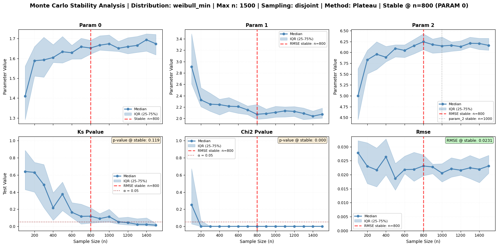
Comparing Stability Detection Methods

The monte_carlo_fit() method supports multiple algorithms for detecting when parameters and goodness-of-fit metrics stabilize. Each method has strengths for different types of metrics. Let’s explore them!

Available Methods:

1. CV (Coefficient of Variation) - Default, robust for all metrics

2. Kneedle Algorithm - Best for decreasing metrics (RMSE) and converging parameters

3. Plateau Detection - Good for metrics with clear convergence behavior

Let’s compare these methods using our large dataset.

# Test all three stability detection methods
print("Comparing Stability Detection Methods")
print("=" * 80)
print("Running Monte Carlo analysis with different detection methods...")
print("This will take a moment...\n")

# Common parameters for all methods
common_params = {
    'sizes': np.arange(100, 1600, 100),
    'n_repeats': 30,
    'tests': ['ks', 'chi2', 'rmse'],
    'sampling': 'disjoint',
    'seed': 42,
    'plot_type': 'series'
}

# Dictionary to store results
method_results = {}
method_names = {
    'cv': 'Coefficient of Variation',
    'kneedle': 'Kneedle Algorithm',
    'plateau': 'Plateau Detection'
}

# Run analysis with each method
for method_key in ['cv', 'kneedle', 'plateau']:
    print(f"Running with {method_names[method_key]}...")

    print(f"\n{method_names[method_key]}:")
    print("-" * 80)
    fig_path = f'mc_method_{method_key}.png'

    results = large_processor.monte_carlo_fit(
        **common_params,
        stability_method=method_key,
        fig_output_path=fig_path
    )

    method_results[method_key] = results
    print(f"  ✓ Completed - Figure saved to: {fig_path}\n")

print("\n" + "=" * 80)
print("FIGURE INTERPRETATION:")
print("=" * 80)
print("\n🔍 What to Look For:")
print("\n1. Red Dashed Vertical Lines**: Detected stability points")
print("   • Shows where each variable stabilizes according to the method")
print("   • Different methods may place these at different locations")
print("\n2. **Orange Dashed Lines** (Kneedle only): Smoothed median curve")
print("   • Helps identify the 'elbow' point more clearly")
print("   • Only visible when using Kneedle method with smoothing enabled")
print("\n3. **RMSE Panel** (Bottom Right):")
print("   • Typically shows clearest convergence behavior")
print("   • Kneedle excels at finding the elbow in this curve")
print("   • Look for where the curve flattens out")
print("\n4. **Parameter Panels** (Top Row):")
print("   • Should show convergence as n increases")
print("   • IQR (shaded area) should decrease")
print("   • Plateau detection works well here")
print("\n5. **P-value Panels** (Bottom Left/Center):")
print("   • Red dotted horizontal line at α = 0.05")
print("   • Text box shows p-value at stable point")
print("   • Can be erratic - CV method handles variability best")

Comparing Stability Detection Methods
================================================================================
Running Monte Carlo analysis with different detection methods...
This will take a moment...

Running with Coefficient of Variation...

Coefficient of Variation:
--------------------------------------------------------------------------------

Monte Carlo sizes: 100%|██████████| 15/15 [00:08<00:00,  1.72it/s]

  ✓ Completed - Figure saved to: mc_method_cv.png

Running with Kneedle Algorithm...

Kneedle Algorithm:
--------------------------------------------------------------------------------

Monte Carlo sizes: 100%|██████████| 15/15 [00:09<00:00,  1.55it/s]

  ✓ Completed - Figure saved to: mc_method_kneedle.png

Running with Plateau Detection...

Plateau Detection:
--------------------------------------------------------------------------------

Monte Carlo sizes: 100%|██████████| 15/15 [00:09<00:00,  1.59it/s]

  ✓ Completed - Figure saved to: mc_method_plateau.png


================================================================================
FIGURE INTERPRETATION:
================================================================================

🔍 What to Look For:

1. Red Dashed Vertical Lines**: Detected stability points
   • Shows where each variable stabilizes according to the method
   • Different methods may place these at different locations

2. **Orange Dashed Lines** (Kneedle only): Smoothed median curve
   • Helps identify the 'elbow' point more clearly
   • Only visible when using Kneedle method with smoothing enabled

3. **RMSE Panel** (Bottom Right):
   • Typically shows clearest convergence behavior
   • Kneedle excels at finding the elbow in this curve
   • Look for where the curve flattens out

4. **Parameter Panels** (Top Row):
   • Should show convergence as n increases
   • IQR (shaded area) should decrease
   • Plateau detection works well here

5. **P-value Panels** (Bottom Left/Center):
   • Red dotted horizontal line at α = 0.05
   • Text box shows p-value at stable point
   • Can be erratic - CV method handles variability best

# Compare stability points detected by each method
print("STABILITY POINT COMPARISON")
print("=" * 90)
print(f"{'Method':<25} {'RMSE':<15} {'KS p-value':<15} {'Chi² p-value':<15} {'Param 0':<15}")
print("-" * 90)

for method_key, method_name in method_names.items():
    results = method_results[method_key]
    stability = results.attrs['stability_points']

    rmse_size = stability.get('rmse', {}).get('size', 'Not detected')
    ks_size = stability.get('ks_pvalue', {}).get('size', 'Not detected')
    chi2_size = stability.get('chi2_pvalue', {}).get('size', 'Not detected')
    param0_size = stability.get('param_0', {}).get('size', 'Not detected')

    print(f"{method_name:<25} {str(rmse_size):<15} {str(ks_size):<15} {str(chi2_size):<15} {str(param0_size):<15}")

print("\n" + "=" * 90)
print("RECOMMENDED SIZES")
print("=" * 90)

for method_key, method_name in method_names.items():
    results = method_results[method_key]
    recommended = results.attrs.get('recommended_size', 'N/A')
    primary = results.attrs.get('primary_metric', 'N/A')

    print(f"{method_name:<25} n = {recommended:<10} (based on {primary})")

print("\n💡 KEY OBSERVATIONS:")
print("   • Different methods may detect different stability points")
print("   • RMSE typically shows clearest stability (especially with Kneedle)")
print("   • P-values can be more variable - CV method handles this well")
print("   • Kneedle excels at finding the 'elbow' in decreasing curves")
print("   • Plateau works well when improvement becomes negligible")

STABILITY POINT COMPARISON
==========================================================================================
Method                    RMSE            KS p-value      Chi² p-value    Param 0
------------------------------------------------------------------------------------------
Coefficient of Variation  None            None            3000            1600
Kneedle Algorithm         400             1200            400             400
Plateau Detection         None            None            2500            2500

==========================================================================================
RECOMMENDED SIZES
==========================================================================================
Coefficient of Variation  n = 3000       (based on chi2_pvalue)
Kneedle Algorithm         n = 400        (based on rmse)
Plateau Detection         n = 2500       (based on chi2_pvalue)

💡 KEY OBSERVATIONS:
   • Different methods may detect different stability points
   • RMSE typically shows clearest stability (especially with Kneedle)
   • P-values can be more variable - CV method handles this well
   • Kneedle excels at finding the 'elbow' in decreasing curves
   • Plateau works well when improvement becomes negligible

Understanding Each Method

1. Coefficient of Variation (CV) Method

How it works:

• Calculates std/mean across repeats for each sample size

• Looks for when CV stays consistently below 10% threshold

• Uses a sliding window to ensure stability is sustained

Best for:

• General purpose - works for all metrics

• P-values (which can be erratic)

• When you need robust, conservative estimates

Parameters:

• window_size: Number of consecutive sizes that must be stable (default: len(sizes)//4)

• cv_threshold: Maximum acceptable CV (default: 0.1 = 10%)

2. Kneedle Algorithm

How it works:

• Based on Satopää et al. (2011) paper

• Normalizes curve to [0,1] range

• Finds maximum distance between curve and reference line (the “elbow”)

• Optionally smooths curve first for clearer detection

Best for:

• RMSE (decreasing curves with clear elbow)

• Converging parameters

• When you want to find the “point of diminishing returns”

Parameters:

• smooth: Enable curve smoothing (default: True)

• smoothing_method: ‘savgol’ (default) or ‘spline’

Visual indicator:

• Orange dashed line shows smoothed curve in figures

3. Plateau Detection

How it works:

• Uses relative gain heuristic: Δᵢ = |y(i-1) - y(i)| / |y(i-1)|

• Detects when improvement becomes negligible

• Requires several consecutive points below threshold

Best for:

• Converging parameters

• Metrics with clear plateau behavior

• When you want early detection of “good enough”

Parameters:

• consecutive_points: L parameter - points that must satisfy criterion (default: 3)

• relative_tolerance: Δ parameter - maximum acceptable change (default: 0.01 = 1%)

# Demonstrate method-specific parameters
print("TESTING METHOD-SPECIFIC PARAMETERS")
print("=" * 80)
print("\nLet's see how parameter tuning affects detection...\n")

# Test Kneedle with different smoothing methods
print("1. Kneedle with different smoothing:")
print("-" * 40)

for smooth_method in ['savgol', 'spline']:
    results_smooth = large_processor.monte_carlo_fit(
        sizes=[100, 400, 800, 1500, 2500, 4000],
        n_repeats=20,
        tests=['rmse'],
        stability_method='kneedle',
        smooth=True,
        smoothing_method=smooth_method,
        seed=42
    )

    rmse_stable = results_smooth.attrs['stability_points']['rmse']['size']
    print(f"  {smooth_method:8s}: RMSE stabilizes at n = {rmse_stable}")

# Test Plateau with different tolerances
print("\n2. Plateau with different relative tolerances:")
print("-" * 40)

for tol in [0.005, 0.01, 0.02]:
    results_plateau = large_processor.monte_carlo_fit(
        sizes=[100, 400, 800, 1500, 2500, 4000],
        n_repeats=20,
        tests=['rmse'],
        stability_method='plateau',
        relative_tolerance=tol,
        consecutive_points=3,
        seed=42
    )

    rmse_stable = results_plateau.attrs['stability_points']['rmse'].get('size', 'Not detected')
    print(f"  Δ = {tol:.3f} (tol = {tol*100:.1f}%): RMSE stabilizes at n = {rmse_stable}")

# Test CV with different thresholds
print("\n3. CV with different thresholds:")
print("-" * 40)

for cv_thresh in [0.05, 0.10, 0.15]:
    results_cv = large_processor.monte_carlo_fit(
        sizes=[100, 400, 800, 1500, 2500, 4000],
        n_repeats=20,
        tests=['rmse'],
        stability_method='cv',
        cv_threshold=cv_thresh,
        seed=42
    )

    rmse_stable = results_cv.attrs['stability_points']['rmse'].get('size', 'Not detected')
    print(f"  CV < {cv_thresh:.2f} ({cv_thresh*100:.0f}%): RMSE stabilizes at n = {rmse_stable}")

print("\n💡 KEY INSIGHTS:")
print("   • Stricter thresholds → Later detection (more conservative)")
print("   • Looser thresholds → Earlier detection (more aggressive)")
print("   • Savgol smoothing preserves features better than spline")
print("   • Choose parameters based on your application's needs")

TESTING METHOD-SPECIFIC PARAMETERS
================================================================================

Let's see how parameter tuning affects detection...

1. Kneedle with different smoothing:
----------------------------------------

Monte Carlo sizes: 100%|██████████| 6/6 [00:02<00:00,  2.09it/s]

  savgol  : RMSE stabilizes at n = 800

Monte Carlo sizes: 100%|██████████| 6/6 [00:03<00:00,  1.77it/s]

  spline  : RMSE stabilizes at n = 1500

2. Plateau with different relative tolerances:
----------------------------------------

Monte Carlo sizes: 100%|██████████| 6/6 [00:02<00:00,  2.05it/s]

  Δ = 0.005 (tol = 0.5%): RMSE stabilizes at n = None

Monte Carlo sizes: 100%|██████████| 6/6 [00:02<00:00,  2.14it/s]

  Δ = 0.010 (tol = 1.0%): RMSE stabilizes at n = None

Monte Carlo sizes: 100%|██████████| 6/6 [00:02<00:00,  2.01it/s]

  Δ = 0.020 (tol = 2.0%): RMSE stabilizes at n = None

3. CV with different thresholds:
----------------------------------------

Monte Carlo sizes: 100%|██████████| 6/6 [00:02<00:00,  2.08it/s]

  CV < 0.05 (5%): RMSE stabilizes at n = None

Monte Carlo sizes: 100%|██████████| 6/6 [00:02<00:00,  2.03it/s]

  CV < 0.10 (10%): RMSE stabilizes at n = None

Monte Carlo sizes: 100%|██████████| 6/6 [00:02<00:00,  2.11it/s]

  CV < 0.15 (15%): RMSE stabilizes at n = 2500

💡 KEY INSIGHTS:
   • Stricter thresholds → Later detection (more conservative)
   • Looser thresholds → Earlier detection (more aggressive)
   • Savgol smoothing preserves features better than spline
   • Choose parameters based on your application's needs

Method Selection Guide

Use this table to choose the best method for your analysis:

Your Metric	Recommended Method	Why
RMSE	kneedle	Clear decreasing curve with distinct elbow point
Parameters (converging)	kneedle or plateau	Both work well for convergence detection
KS p-value	cv	Can be erratic; CV handles variability robustly
Chi² p-value	cv	Can be erratic; CV handles variability robustly
Mixed metrics	cv	General purpose, works for everything
Need early detection	plateau	Detects “good enough” earlier
Need conservative estimate	cv	More stringent criteria

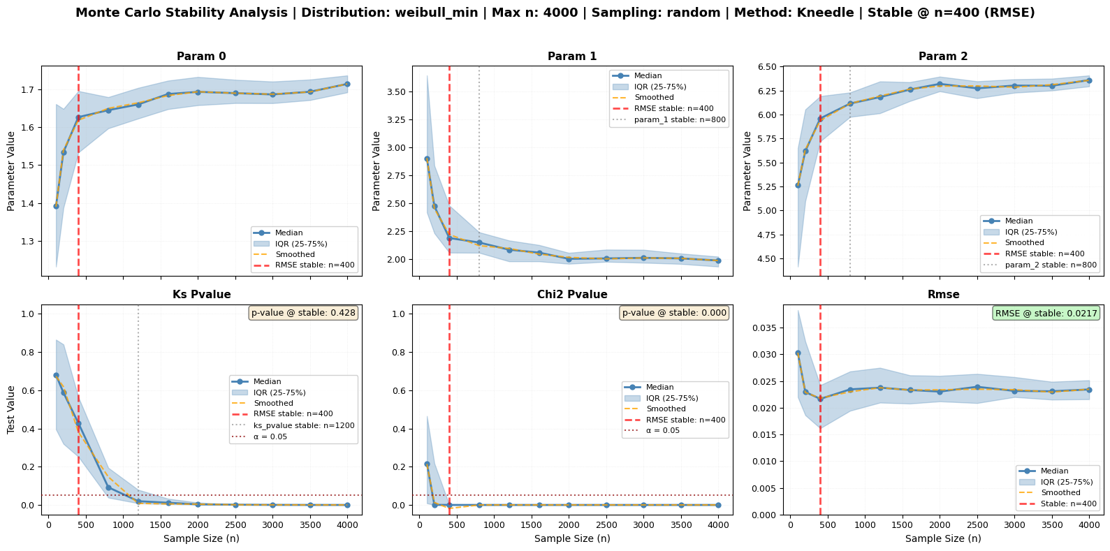
from IPython.display import Image, display

# Practical example: Use the best method for RMSE
print("PRACTICAL EXAMPLE: Using Kneedle for RMSE Analysis")
print("=" * 80)
print("\nThis is the recommended approach for most cases.\n")

# Run with Kneedle method
final_results = large_processor.monte_carlo_fit(
    sizes=[100, 200, 400, 800, 1200, 1600, 2000, 2500, 3000, 3500, 4000],
    n_repeats=50,
    tests=['ks', 'chi2', 'rmse'],
    stability_method='kneedle',
    smooth=True,
    smoothing_method='savgol',
    sampling='random',
    seed=42,
    fig_output_path='final_stability_analysis.png',
    plot_type='series'
)

# Extract key information
recommended_n = final_results.attrs['recommended_size']
primary_metric = final_results.attrs['primary_metric']
stability_points = final_results.attrs['stability_points']

print("RESULTS:")
print("-" * 80)
print(f"Recommended sample size: n = {recommended_n}")
print(f"Based on: {primary_metric.upper()}")
print(f"\nStability points by metric:")

for metric in ['rmse', 'ks_pvalue', 'chi2_pvalue', 'param_0']:
    if metric in stability_points:
        info = stability_points[metric]
        size = info.get('size', 'Not detected')
        method = info.get('method', 'N/A')
        print(f"  {metric:15s}: n = {size:10} (method: {method})")

# Display quality metrics at stable point
print(f"\nQuality at stable point (n = {recommended_n}):")
if final_results.attrs.get('stable_rmse') is not None:
    print(f"  RMSE:        {final_results.attrs['stable_rmse']:.6f}")
if final_results.attrs.get('stable_pvalue_ks') is not None:
    print(f"  KS p-value:  {final_results.attrs['stable_pvalue_ks']:.4f}")
if final_results.attrs.get('stable_pvalue_chi2') is not None:
    print(f"  χ² p-value:  {final_results.attrs['stable_pvalue_chi2']:.4f}")

print(f"\nFigure saved to: {final_results.attrs['figure_path']}")

# Display the final figure
print("\n" + "=" * 80)
display(Image(filename=final_results.attrs['figure_path']))

print("\n✅ SUCCESS!")
print("   This figure shows:")
print("   • Orange dashed lines: Smoothed curves (Kneedle's preprocessing)")
print("   • Red vertical lines: Detected stability points")
print("   • Informative title: Distribution, max n, and recommended stable point")
print("   • Quality metrics: P-values and RMSE at the stable point")
print(f"\n   Use n = {recommended_n} for robust inference!")

PRACTICAL EXAMPLE: Using Kneedle for RMSE Analysis
================================================================================

This is the recommended approach for most cases.

Monte Carlo sizes:   0%|          | 0/11 [00:00<?, ?it/s]/Users/danilocoutodesouza/miniconda3/envs/magica/lib/python3.11/site-packages/scipy/stats/_stats_py.py:7400: RuntimeWarning: divide by zero encountered in divide
  terms = (f_obs - f_exp)**2 / f_exp
Monte Carlo sizes: 100%|██████████| 11/11 [00:16<00:00,  1.53s/it]

RESULTS:
--------------------------------------------------------------------------------
Recommended sample size: n = 400
Based on: RMSE

Stability points by metric:
  rmse           : n =        400 (method: kneedle)
  ks_pvalue      : n =       1200 (method: kneedle)
  chi2_pvalue    : n =        400 (method: kneedle)
  param_0        : n =        400 (method: kneedle)

Quality at stable point (n = 400):
  RMSE:        0.021654
  KS p-value:  0.4281
  χ² p-value:  0.0000

Figure saved to: final_stability_analysis.png

================================================================================

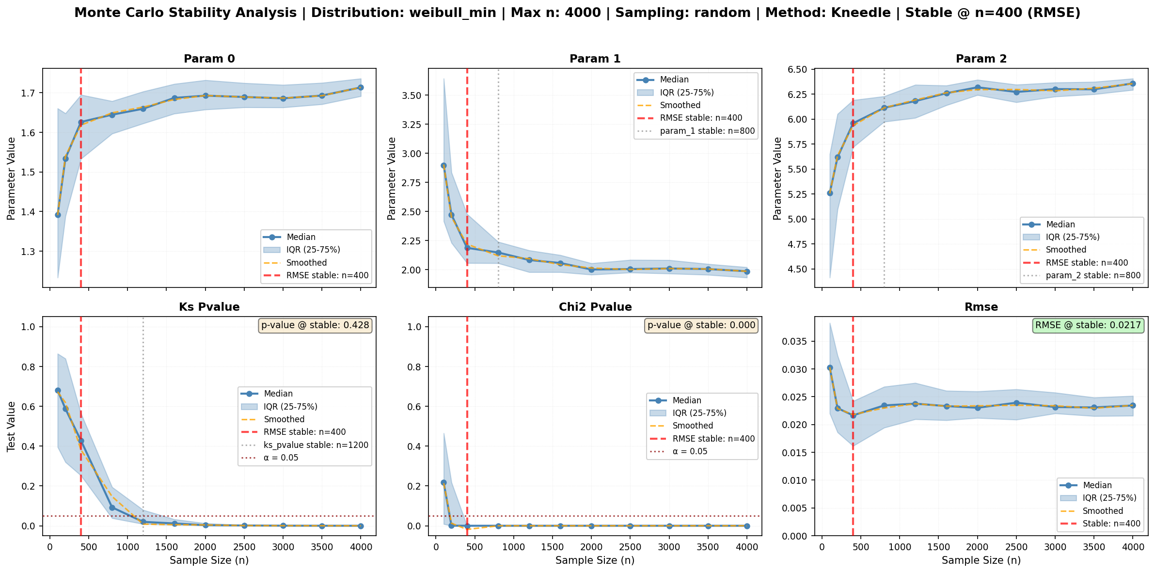
✅ SUCCESS!
   This figure shows:
   • Orange dashed lines: Smoothed curves (Kneedle's preprocessing)
   • Red vertical lines: Detected stability points
   • Informative title: Distribution, max n, and recommended stable point
   • Quality metrics: P-values and RMSE at the stable point

   Use n = 400 for robust inference!

Summary and Best Practices

Key Points:

1. Data Loading: Use ma.read_data() to create a DataProcessor

2. Distribution Fitting: Use .fit_distribution(distribution_name)

3. Direct Method Access: All SciPy methods available directly (pdf, cdf, ppf, etc.)

4. Smart Defaults: Methods like pdf() and cdf() use original data when no input provided

5. Goodness-of-Fit: Use .goodness_of_fit() with ‘ks’, ‘chi2’, or ‘rmse’

6. Bin Selection: Chi-square test supports multiple binning methods (‘doane’, ‘sturges’, etc.)

7. Constraints: Pass fitting constraints as keyword arguments (e.g., floc=0)

8. Stability Analysis: Use monte_carlo_fit() with automatic figure generation

9. Large Sample Effects: For n>5000, use Monte Carlo CPS method to avoid p-value inflation

10. ⭐ RMSE for Stability: RMSE shows clearest convergence - use it as primary stability indicator

Important Considerations:

• ⭐ RMSE: typically shows much clearer convergence than p-values

  • P-values can be erratic and unreliable for stability detection

  • RMSE decreases smoothly and shows clear stabilization points

  • Always include ‘rmse’ in your tests list for Monte Carlo analysis

• Chi-square binning: Different methods can significantly affect results - choose appropriately

• Large samples: P-values become unreliable with very large datasets (n>10,000)

• CPS method: Helps separate statistical significance from practical significance

• Sampling strategy:

  • ‘random’: general purpose, independent draws

  • ‘bootstrap’: with replacement, good for uncertainty estimation

  • ‘disjoint’: non-overlapping, better for temporal/spatial data

• Reproducibility: Always set random seeds for Monte Carlo analyses

• Automatic plotting: Use fig_output_path parameter to generate publication-ready figures

• Plot types: ‘series’ shows medians with IQR, ‘boxplots’ shows distribution per size

Monte Carlo Analysis Features:

The monte_carlo_fit() method provides:

1. Automatic figure generation: Set fig_output_path to save a 2x3 summary plot

2. Stability detection: Automatically identifies where parameters/tests stabilize

3. Multiple tests: Run KS, Chi-square, and RMSE tests simultaneously

4. Flexible sampling: Choose between random, bootstrap, or disjoint strategies

5. Parameter tracking: Monitor how all distribution parameters evolve with sample size

6. Recommended size: Get a suggested optimal subsample size based on stability

🎯 Best Practice - Stability Detection:

Use RMSE as your primary stability indicator:

1. RMSE shows smooth, monotonic decrease as sample size increases

2. Stabilization point is clearly visible (when curve flattens)

3. More reliable than p-values which can fluctuate

4. Directly measures fit quality improvement

Visual cue in plots:

• Look at bottom-right panel (RMSE)

• Find where curve flattens (red dashed line)

• This is your optimal sample size!

For automatic distribution selection, see the AutoFitter tutorial!